This post has a protocol for putting DeepLabCut into GPU server production on github.

1. Using DeepLabCut to perform markless body tracking in mice

DeepLabCut is an open source machine vision package developed in Professor Mackenzie Mathis’s lab at EPFL and Harvard to harness two elements of machine vision into one tool. Firstly, they use convolutional neural networks (CNNS) to learn how to identify different parts of an object using image patches drawn from a single video frame. Next, they use that identification to then find all matching parts in a new video frame and extract the 2D coordinates of the matching parts. So for example, after manually marking a few dozen frames with coordinates for a mouse’s nose, tail tip, left and right hind paws, etc. DeepLabCut will quickly begin to identify the correct location of these parts in any new video run through the algorithm (tens of thousands of frames). This becomes incredibly powerful in basic neuroscience research, where tracking animal movements and behaviors can then be linked to activity in the nervous system and can help better define elements of disease. I am a researcher studying the neural circuit basis of Parkinsonism in mouse models of the disease, so accurately tracking mouse motor behavior is critical.

2. Training a good tracking model on a local computer with GPU

To train the model, you first need some representative example data. This requires thinking about all the major sources of variability you might have: different backgrounds? Different lighting? Different objects that might obscure the image? Different subjects? In my case, I had all of these! In addition I also had video from two different resolution cameras and either in color or B&W video. So I made sure to include example frames of each of these conditions to start with.

The experience of labeling frames is a bit mind numbing but can be fun. (Those immediately interested can see what the experience is like by labeling some animal datasets hosted online). DLC comes with some good Jupyter Notebook examples (e.g. Demo_labeledexample_Openfield.ipynb) that show how to extract example frames from one or more videos, and then use the included GUI to label the mouse body parts in each frame.

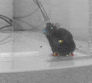
The process of hand labeling forces you to appreciate the possible difficulties the algorithm might also encounter in the data. In my case, we have a lot of data collected on low resolution cameras, and it could be surprisingly difficult to identify all of the mouse bodyparts accurately using the same criteria for each frame when the mouse was in the far corner, facing away.

Higher resolution images were much easier to mark correctly, especially if mouse was close to the camera and not facing away from the camera.

DeepLabCut is designed for this process to be iterative: you select some frames, train the model, check for frames likely to have mistakes (deviate greatly from nearby frames), put markers on the mistaken frames, train again, etc. The process is very similar for adding brand new conditions to an existing model, or tracking new body parts that were not previously labeled. So the strength of the iterations is that it adds a lot of important flexibility. Side note on adding body parts: make sure that the column order doesn’t change in your training set! That happened to me when I added a new body part to the model and it took a bit of time to realize this was the issue.

The downside of the iterations is that you might need quite a few to get something that works reasonably well across really diverse conditions. I ended up needing about 10 iterations, adding around 50 frames each time to get usable data (495 frames total). But some of those iterations were also to add new body parts or new environments.

Overall the tracking got pretty consistent. It’s not perfect (still needs some pre-processing, covered in Part 2 of this series), but this was a good enough start for my purposes, and took less than a day of my time to get the tracking to this point . In this case, each iteration trained for about 1 million cycles overnight on a single GeForce RTX 2070 GPU.

3. Scaling processing to a GPU cluster for production

So now that I had a reasonable model for tracking body coordinates, I had a lot of videos to process. Processing these data on a single GPU takes close to real-time, so a 30 minute video takes approximately 30 minutes to process. I have +1,000 hours of video from more than 1,000 experiments, which means one pass of the processing would take 42 days. Instead, I did it in 2 days. Here’s how!

Carnegie Mellon University has a close relationship with the Pittsburgh Super Computer, and I was able to get a starter grant funded for about 1500 hours of compute time on their GPU nodes. That was just about all I needed to get through my backlog of videos and test out a production for scaling up processing using DeepLabCut.

The full protocol is available here: https://github.com/KidElectric/dlc_protocol but in brief:

1. I realized that an easy approach would be to put DeepLabCut into a container. In essence, a container is like an entire computer in software form: all the files are in place and all it needs is a place to run. In this case, many places to run (in parallel). The PSC GPU nodes were set up to use Singularity images, which are similar to docker containers. So I found an existing docker image, made a few changes, and found the method for importing it to the supercomputer as a singularity image.

module load singularity
singularity build dlc_217.simg docker://kidelectric/deeplabcut:ver2_1_7
#Then, for example, you can run a Linux shell from inside that image:
singularity shell dlc_217.simg

2. I wrote a protocol for uploading all of my videos to the supercomputer using ssh and uploaded the trained DLC model onto the supercomputer.

3. Three scripts were necessary to make the process work in parallel. The trick was to use the SLUM job array call on the supercomputer–this method automatically sends your singularity image out to as many nodes as become available and starts processing new data. So for that I needed: 1) a SLURM job script to initialize the Singularity images and pass the Job ID 2) a Linux .sh script to start python in the image and pass the job ID along and 3) a python script to run inside the Singularity image to translate the SLURM job ID into a video file to analyze and send that to DeepLabCut to begin processing. It also became useful to write code that checked that all videos were processed correctly.

4. Conclusion

This method allowed me to analyze MANY videos simultaneously. Nodes become available whenever other jobs are finished, at certain points I remember seeing a dozens jobs running simultaneously, and sometimes many dozen! Altogether it took about 2 days to analyze the 1,000 hour backlog. That’s a 20x improvement over running on a single GPU computer.

Would it be possible to analyze 1000 hours of video on a single GPU PC? Certainly. However, waiting 42 days is a big risk to take if you might find out that something didn’t work correctly. And it becomes even worse still if you realize the model needs to improve under a new condition. Lastly, if a lab ever wanted to scale up towards a full pipeline, it would only take a few more lines of code: check the lab server for new videos, send them to the supercomputer! Now that I’ve typed that out, maybe I’ll do that this afternoon ;-).

Next up, now that we have some tracking coordinates, what do we do with them??? Part 2: Pre-processing the data. Part 3: classifying the data. Part 4: verification and final tweaks!